resolution

library(obisindicators)
library(dplyr)
#> 
#> Attaching package: 'dplyr'
#> The following objects are masked from 'package:stats':
#> 
#>     filter, lag
#> The following objects are masked from 'package:base':
#> 
#>     intersect, setdiff, setequal, union
library(dggridR) # remotes::install_github("r-barnes/dggridR")
#> Loading required package: rlang
#> Loading required package: sf
#> Linking to GEOS 3.8.0, GDAL 3.0.4, PROJ 6.3.1; sf_use_s2() is TRUE
#> Loading required package: sp
library(sf)

Get biological occurrences

occ <- occ_SAtlantic # occ_1M OR occ_SAtlantic

Create function to make grid, calculate metrics, and plot maps for different resolution grid sizes

res_changes <- function(resolution = 9){
    dggs <- dgconstruct(projection = "ISEA", topology = "HEXAGON", res = resolution)
    occ$cell <- dgGEO_to_SEQNUM(dggs, occ$decimalLongitude, occ$decimalLatitude)[["seqnum"]]
    idx <- calc_indicators(occ)

  grid <- dgcellstogrid(dggs, idx$cell) %>% 
    st_wrap_dateline() %>% 
    rename(cell = seqnum) %>% 
    left_join(
      idx,
      by = "cell")

  gmap_indicator(grid, "es", label = "ES(50)")
}

Different Resolutions

Here we plot res 4, which has hex areas of ~630,000 sq km This is the highest resolution we can plot without having gaps in the Central Atlantic Region

res_changes(4)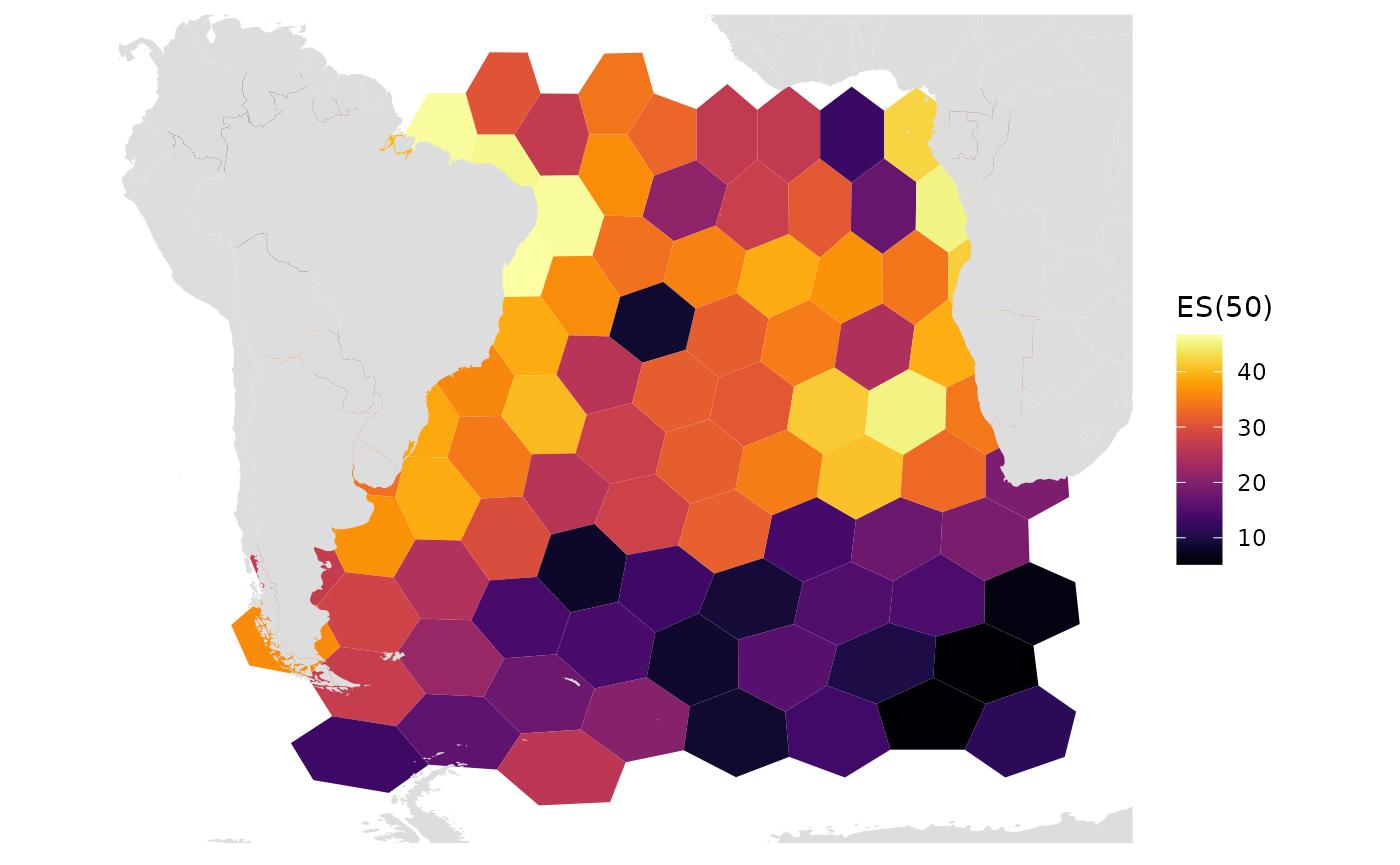

Here we plot res 6, which has hex areas of ~70,000 sq km.

We still see some gaps and can begin to see the band of high amounts of sampling towards the bottom This can show us where more sampling is needed

res_changes(6)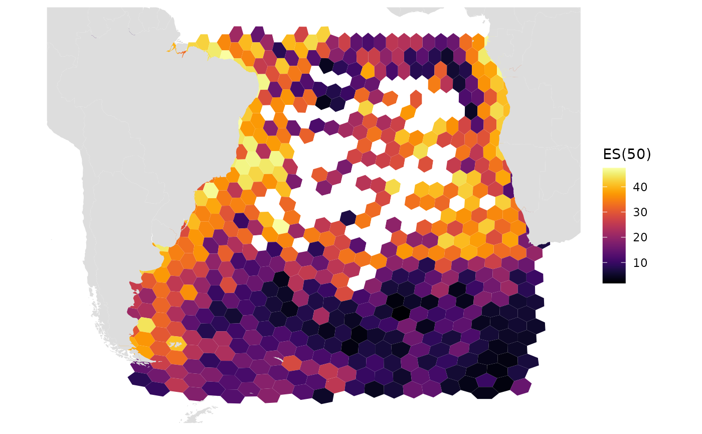

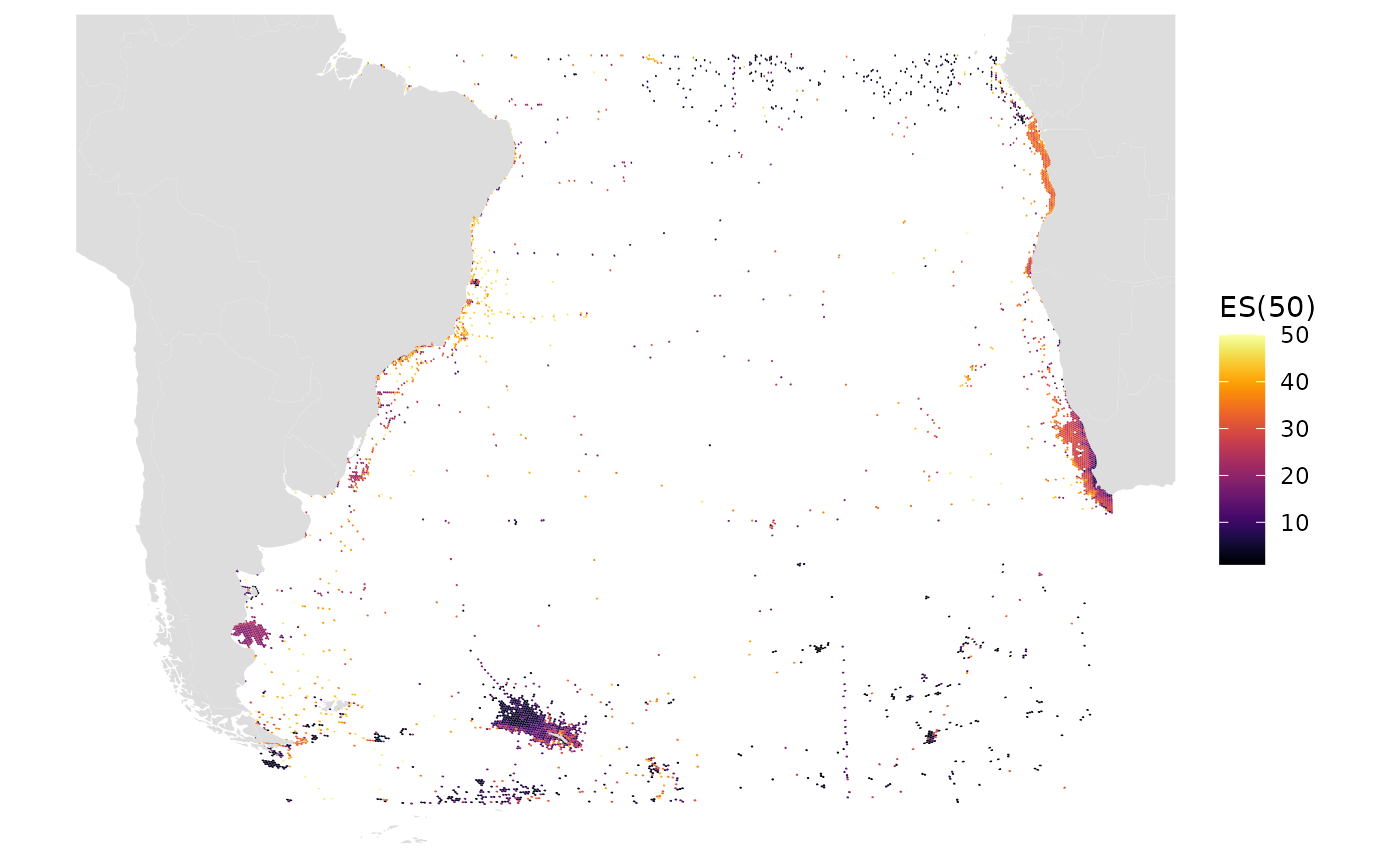
Here we plot res 9, which has hex areas of ~2600 sq km, the default resolution

res_changes(9)

Here we plot res 11, which has hex areas of ~288 sq km

We see a large amount of gaps throughout the South Atlantic when we get down to this small area

res_changes(11)