Get biological occurrences
Use the 1 million records subsampled from the full OBIS dataset otherwise available at https://obis.org/data/access.
occ <- occ_1M # occ_1M OR occ_SAtlanticCreate a discrete global grid
Create an ISEA discrete global grid of resolution 9 using the dggridR package:
library(dggridR) # remotes::install_github("r-barnes/dggridR")

dggs <- dgconstruct(projection = "ISEA", topology = "HEXAGON", res = 9)
Here’s on overview of all possible resolutions specified by the res parameter above:
inf <- dginfo(dggs)
#>    res            cells                area_km      spacing_km          cls_km
#> 1    0               12 51006562.1724088639021 7053.6524314108 8199.5003701020
#> 2    1               32 17002187.3908029571176 4072.4281300451 4678.9698717297
#> 3    2               92  5667395.7969343187287 2351.2174771369 2691.2520709129
#> 4    3              272  1889131.9323114394210 1357.4760433484 1551.8675487723
#> 5    4              812   629710.6441038132180  783.7391590456  895.6018416484
#> 6    5             2432   209903.5480346043769  452.4920144495  517.0049969031
#> 7    6             7292    69967.8493448681256  261.2463863485  298.4793231872
#> 8    7            21872    23322.6164482893764  150.8306714832  172.3244908961
#> 9    8            65612     7774.2054827631255   87.0821287828   99.4910857272
#> 10   9           196832     2591.4018275877083   50.2768904944   57.4411078487
#> 11  10           590492      863.8006091959028   29.0273762609   33.1636203580
#> 12  11          1771472      287.9335363986343   16.7589634981   19.1470215381
#> 13  12          5314412       95.9778454662114    9.6757920870   11.0545373459
#> 14  13         15943232       31.9926151554038    5.5863211660    6.3823399790
#> 15  14         47829692       10.6642050518013    3.2252640290    3.6848456792
#> 16  15        143489072        3.5547350172671    1.8621070553    2.1274466399
#> 17  16        430467212        1.1849116724224    1.0750880097    1.2282818893
#> 18  17       1291401632        0.3949705574741    0.6207023518    0.7091488792
#> 19  18       3874204892        0.1316568524914    0.3583626699    0.4094272963
#> 20  19      11622614672        0.0438856174971    0.2069007839    0.2363829597
#> 21  20      34867844012        0.0146285391657    0.1194542233    0.1364757654
#> 22  21     104603532032        0.0048761797219    0.0689669280    0.0787943199
#> 23  22     313810596092        0.0016253932406    0.0398180744    0.0454919218
#> 24  23     941431788272        0.0005417977469    0.0229889760    0.0262647733
#> 25  24    2824295364812        0.0001805992490    0.0132726915    0.0151639739
#> 26  25    8472886094432        0.0000601997497    0.0076629920    0.0087549244
#> 27  26   25418658283292        0.0000200665832    0.0044242305    0.0050546580
#> 28  27   76255974849872        0.0000066888611    0.0025543307    0.0029183081
#> 29  28  228767924549612        0.0000022296204    0.0014747435    0.0016848860
#> 30  29  686303773648832        0.0000007432068    0.0008514436    0.0009727694
#> 31  30 2058911320946492        0.0000002477356    0.0004915812    0.0005616287
Then assign cell numbers to the occurrence data:
occ$cell <- dgGEO_to_SEQNUM(dggs, occ$decimalLongitude, occ$decimalLatitude)[["seqnum"]]Calculate indicators
The following function calculates the number of records, species richness, Simpson index, Shannon index, Hurlbert index (n = 50), and Hill numbers for each cell.
Perform the calculation on species level data:
idx <- calc_indicators(occ)Add cell geometries to the indicators table (idx):
library(sf)

grid <- dgcellstogrid(dggs, idx$cell) %>%
  st_wrap_dateline() %>%
  rename(cell = seqnum) %>%
  left_join(
    idx,
    by = "cell")
Plot maps of indicators
Let’s look at the resulting indicators in map form.
# ES(50)
gmap_indicator(grid, "es", label = "ES(50)")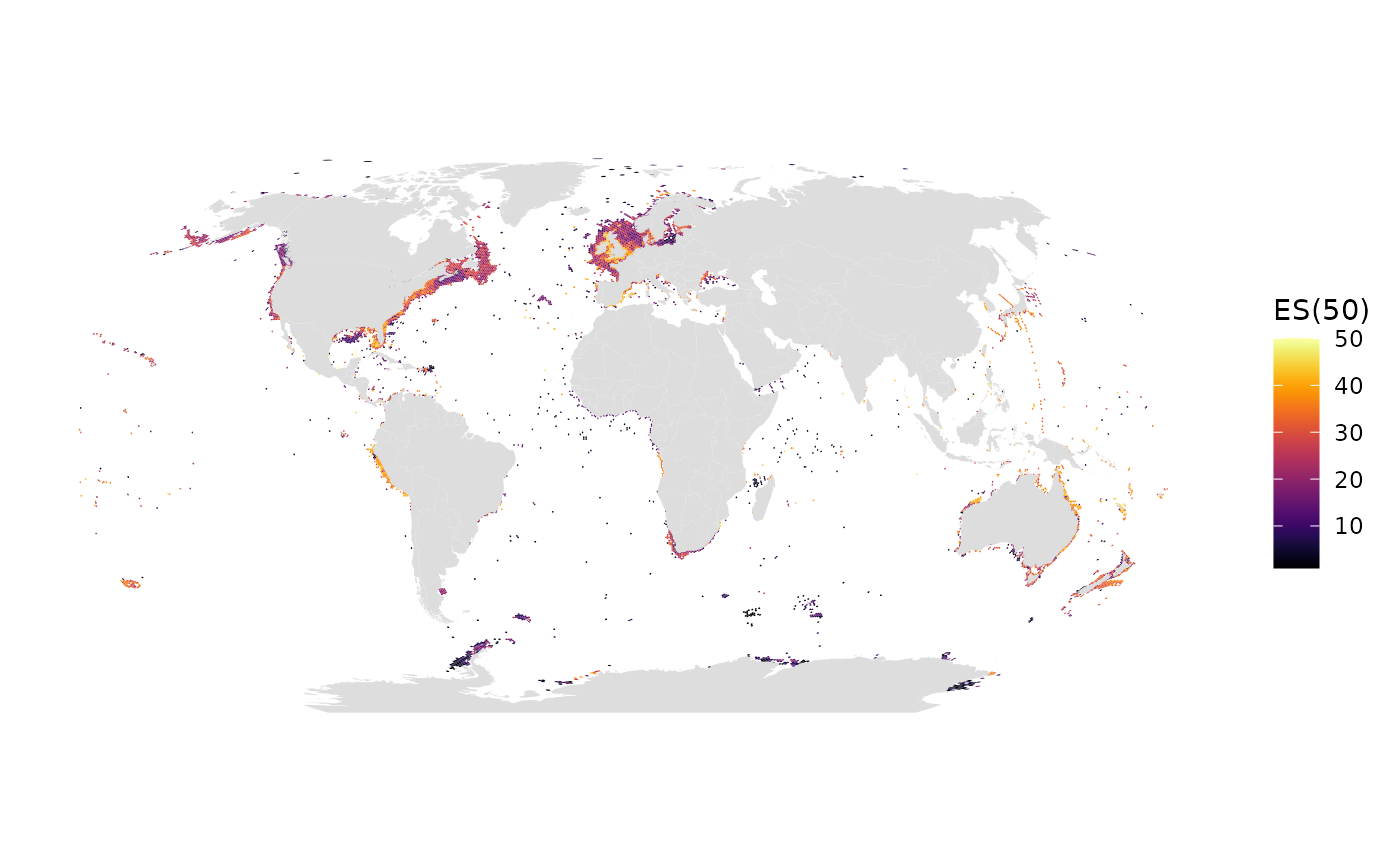
# Shannon index
gmap_indicator(grid, "shannon", label = "Shannon index")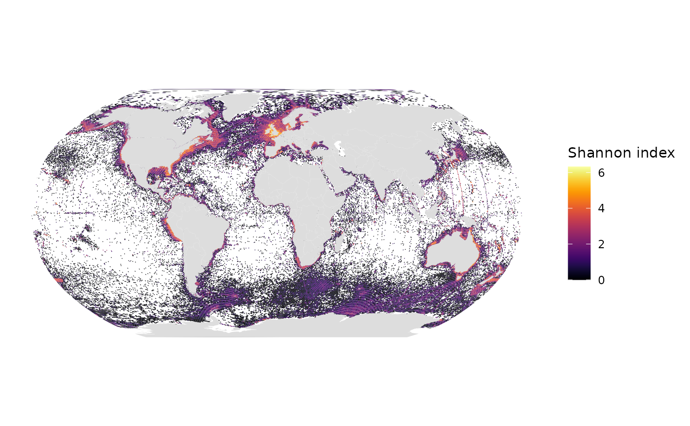
# Number of records, log10 scale, Robinson projection (default)
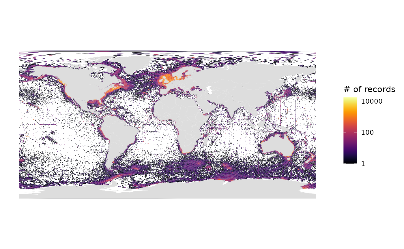
gmap_indicator(grid, "n", label = "# of records", trans = "log10")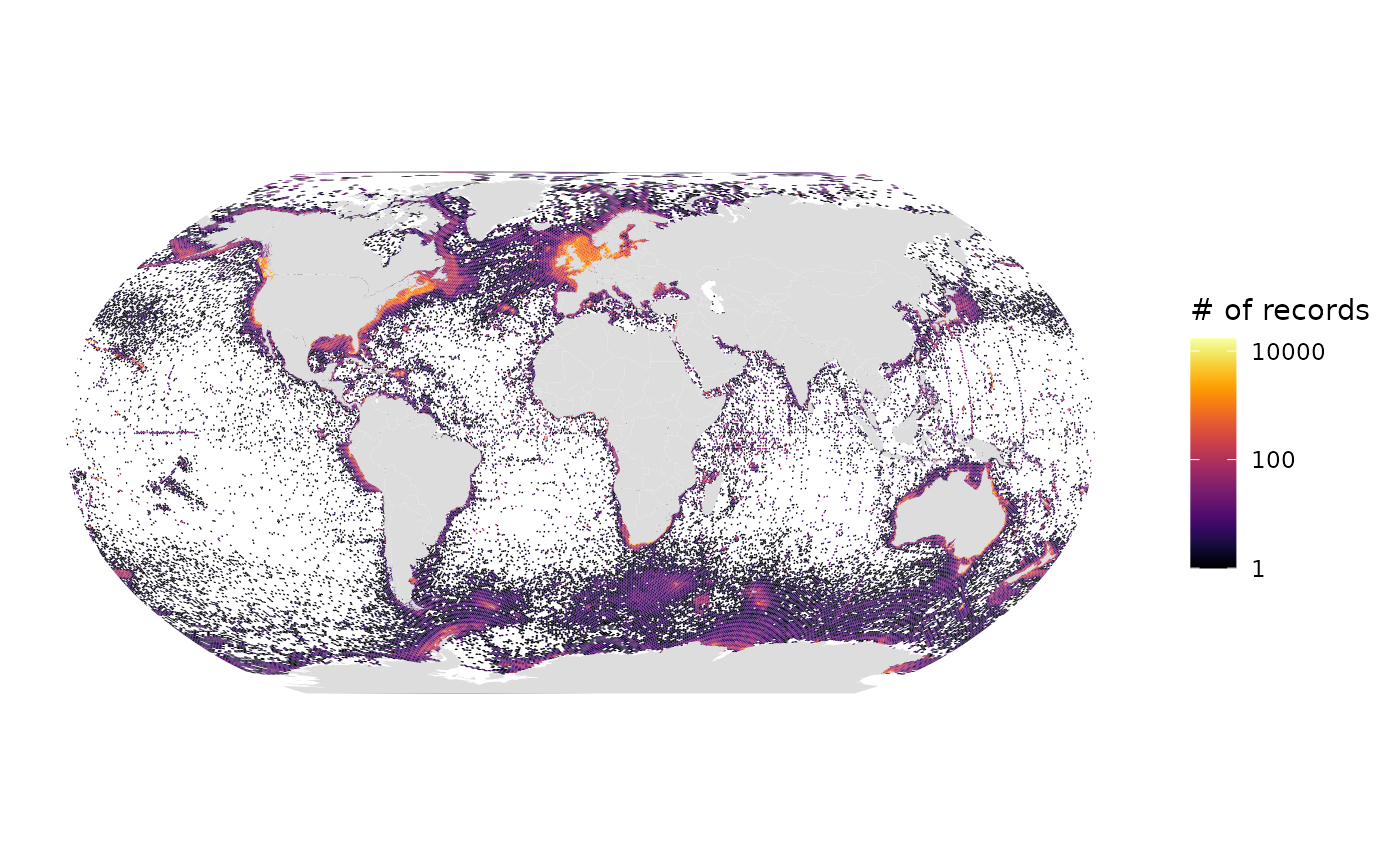
# Number of records, log10 scale, Geographic projection
gmap_indicator(grid, "n", label = "# of records", trans = "log10", crs=4326)