Calculate Indicators

Setup database

Using PostgreSQL with PostGIS extension in Docker:

create volume `pg_data`

docker volume create pg_data

create container `postgis`, database `am` user `admin`

On command line:

# set password as environment variable read in from file
DB_PASS=`cat ~/private/pg_pass`

# run docker with image
docker run --name=postgis \
  -d -e POSTGRES_USER=admin \
  -e POSTGRES_PASS=$DB_PASS \
  -e POSTGRES_DBNAME=am \
  -e ALLOW_IP_RANGE=0.0.0.0/0 \
  -p 5432:5432 \
  -v pg_data:/var/lib/postgresql \
  -v /Users/bbest/docker_pg_data:/data \
  --restart=always \
  --shm-size=1g \
  kartoza/postgis:11.0-2.5

# check logs
docker logs postgis

Connect to database

library(tidyverse)
library(here)
library(glue)
library(raster)
library(DBI)
library(RPostgreSQL)
library(tictoc)
library(furrr)
library(RColorBrewer)

library(devtools); load_all() # library(gmbi)

## ✔ Setting active project to '/Users/bbest/github/gmbi'
## ✔ Saving 'spp' to 'data/spp.rda'
## ✔ Saving 'spp_iucn' to 'data/spp_iucn.rda'

# paths
dir_tmp      <- here("inst/tmp")
dir_out      <- here("inst/data/rasters")
spp_iucn_csv <- here("inst/data/spp_iucn.csv")
spp_csv      <- here("inst/data/spp.csv")
dir_nc       <- "~/docker_pg_data/aquamaps2100_nc"
spp_2100_csv <- "~/docker_pg_data/aquamaps2100_nc.csv"

# plotting parameters
pal <- colorRampPalette(brewer.pal(11, "Spectral"))
cols <- rev(pal(255))
par(mar=c(0.5,0.5,0.5,0.5))

# database connection
con <- get_db_con(password=readLines("~/private/pg_pass"))
con

## <PostgreSQLConnection>

Load AquaMaps csvs into database

All the species distribution data was generously provided as comma-seperated value (csv) files in a zip package aquamaps_ver0816c.zip by Kristin Kaschner and Cristina Garilao to Ben Best ben@ecoquants.com on Jun 21, 2018 from the extensive work available at http://AquaMaps.org to be fully cited (K. Kaschner et al. 2016) whenever used.

Generated here are derived products. Please contact Kristin Kaschner kristin.kaschner@biologie.uni-freiburg.de and Cristina Garilao cgarilao@geomar.de for access to the full database.

csv_to_db(con)

# drop odd columns
dbExecute(con, 'ALTER TABLE spp DROP COLUMN "X11", DROP COLUMN "X12";')

spp <- tbl(con, "spp") %>% 
  collect() %>% 
  mutate(
    genus_species = glue("{Genus} {Species}") %>% as.character())

copy_to(
  con, spp, "spp", temporary=F, overwrite=T,
  unique_indexes=list("SPECIESID"),
  indexes = list("group", "genus_species"))

Load tables for querying.

spp       <- tbl(con, "spp")
cells     <- tbl(con, "cells")
spp_cells <- tbl(con, "spp_cells")
obs_cells <- tbl(con, "obs_cells")

Assign taxonomic groups

Assign taxonomic groups borrowing from previous global OBIS analysis (Tittensor et al. 2010).

Primarily coastal species (Tittensor et al. 2010)
- Coastal fishes: Class == "Actinopterygii" & !Family %in% c("Scombridae", "Istiophoridae", "Xiphiidae")
- Non-oceanic sharks: TODO with rredlist::rl_habitats()
- Non-squid cephalopods: Class == "Cephalopoda" & !Order %in% c("Myopsida","Oegopsida")
- Pinnipeds: Family %in% c("Odobenidae", "Otariidae", "Phocidae")
- Corals: Class == "Anthozoa" (soft/hard + anemones + gorgonians)
- Seagrasses: Order == "Alismatales"
- Mangroves: Genus == "Avicennia" & Species == "germinans" (n=1)
Primarily oceanic species (Tittensor et al. 2010)
- Tunas and billfishes: Family %in% c("Scombridae", "Istiophoridae", "Xiphiidae")
- Oceanic sharks: TODO with rredlist::rl_habitats()
- Squids: Order %in% c("Myopsida","Oegopsida")
- Cetaceans: Order == "Artiodactyla"
- Euphausiids: Order == "Euphausiacea"
- Foraminifera: n=0 for Phylum=Retaria
Others (Phylum - Class)
- Arthropoda
  - Crustaceans: Class %in% c("Malacostraca","Ostracoda","Branchiopoda","Cephalocarida","Maxillopoda")
  - Sea spiders: Class == "Pycnogonida"
  - skipping: Arachnida (1), Merostomata (1)
- Mollusca
  - Gastropods: Class == "Gastropoda"
  - Bivalves: Class == "Bivalvia"
  - Chitons: Class == "Polyplacophora"
  - Cephalopods
  - Squids
- Chordata
  - Tunicates: Class %in% c("Ascidiacea","Thaliacea")
  - Sharks: Class == "Elasmobranchii" (actually Class=Chondrichthyes, Subclass=Elasmobranchii)
  - Reptiles: Class == "Reptilia" crocodiles, sea snakes & sea turtles
- Echinoderms: Phylum == "Echinodermata"
- Sponges: Phylum == "Porifera"
- Worms: Phylum == "Annelida"
- Cnidaria
  - Hydrozoans: Class == "Hydrozoa"

spp_cols <- tbl(con, "spp") %>% head(1) %>% collect() %>% names()

if (!"group" %in% spp_cols){

  spp <- spp %>% 
    mutate(
      group = case_when(
        Class == "Actinopterygii" & !Family %in% c("Scombridae", "Istiophoridae", "Xiphiidae") ~ "Coastal fishes",
        Class == "Cephalopoda" & !Order %in% c("Myopsida","Oegopsida") ~ "Non-squid cephalopods",
        Family %in% c("Odobenidae", "Otariidae", "Phocidae") ~ "Pinnipeds",
        Class == "Anthozoa" ~ "Corals",
        Order == "Alismatales" ~ "Seagrasses",
        Genus == "Avicennia" & Species == "germinans" ~ "Mangroves",
        Family %in% c("Scombridae", "Istiophoridae", "Xiphiidae") ~ "Tunas & billfishes",
        Order %in% c("Myopsida","Oegopsida") ~ "Squids",
        Order == "Artiodactyla" ~ "Cetaceans",
        Order == "Euphausiacea" ~ "Euphausiids",
        Class %in% c("Malacostraca","Ostracoda","Branchiopoda","Cephalocarida","Maxillopoda") ~ "Crustaceans",
        Class == "Pycnogonida" ~ "Sea spiders",
        Class == "Gastropoda" ~ "Gastropods",
        Class == "Bivalvia" ~ "Bivalves",
        Class == "Polyplacophora" ~ "Chitons",
        Class %in% c("Ascidiacea","Thaliacea") ~ "Tunicates",
        Class == "Elasmobranchii" ~ "Sharks",
        Class == "Reptilia"~ "Reptiles",
        Phylum == "Echinodermata"~ "Echinoderms",
        Phylum == "Porifera" ~ "Sponges",
        Phylum == "Annelida" ~ "Worms",
        Class == "Hydrozoa" ~ "Hydrozoans")) %>% 
    collect()
  
  copy_to(
    con, spp, "spp", temporary=F, overwrite=T,
    unique_indexes=list("SPECIESID"),
    indexes = list("group"))
}

spp_group <- tbl(con, "spp") %>% 
  pull(group)
table(spp_group, useNA="always")

Get extinction risk from IUCN

RedList token issued to ben@ecoquants.com via http://apiv3.iucnredlist.org/api/v3/token.

if (!file.exists(spp_iucn_csv)){
  
  # speed up get_iucn() by running 
  # as multi-threaded process w/ furrr::future_map()

  plan(multiprocess)
  
  # get private IUCN RedList token key
  rl_token <- readLines("~/private/iucn_api_key")
  spp <- tbl(con, "spp") %>% collect()

  # iterate in chunks of 1000
  n <- 1000
  for ( i in seq(1, nrow(spp), by=n) ){
    i_beg <- i
    i_end <- i - 1 + n
    csv <- glue("{dir_tmp}/spp_iucn_{str_pad(i_beg, 5, 'left', '0')}-{str_pad(i_end, 5, 'left', '0')}.csv")
    cat(glue("{basename(csv)} - {Sys.time()}\n\n"))
    
    spp_i <- slice(spp, i_beg:i_end)
    tic()  
    spp_i$iucn <- future_map(spp_i$genus_species, get_iucn, key=rl_token)
    toc() # 262.211 sec; 262.211 / 1000 * 24904 / 60 = 108.8 min for all rows
    
    spp_i <- spp_i %>% 
      mutate(
        iucn_category         = map_chr(iucn, "category"),
        iucn_criteria         = map_chr(iucn, "criteria"),
        iucn_population_trend = map_chr(iucn, "population_trend"),
        iucn_published_year   = map_chr(iucn, "published_year")) %>% 
      select(SPECIESID, starts_with("iucn_"))
    
    write_csv(spp_i, csv)
  }

  # consolidate csvs
  csvs <- list.files(dir_tmp, "^spp_iucn_.*", full.names = T)
  df <- map(csvs, function(x) read_csv(x)) %>% bind_rows()
  write_csv(df, csv)
  unlink(dir_tmp, recursive = T)
}
iucn <- read_csv(spp_iucn_csv)

iucn_cols <- iucn %>% select(starts_with("iucn_")) %>% names()
spp_cols <- tbl(con, "spp") %>% head(1) %>% collect() %>% names()
if (!all(iucn_cols %in% spp_cols)){
  # write to db
  spp <- tbl(con, "spp") %>% 
    collect() %>% 
    left_join(df, by="SPECIESID")
  copy_to(
    con, spp, "spp", temporary=F, overwrite=T,
    unique_indexes=list("SPECIESID"),
    indexes = list("group", "genus_species", "iucn_category"))
}

spp_iucn_category <- tbl(con, "spp") %>% 
  pull(iucn_category)
table(spp_iucn_category, useNA="always")

## spp_iucn_category
##    CR    DD    EN    EX    LC LR/cd LR/lc LR/nt    NT    VU  <NA> 
##    42  1034    87     1  6183     3     4     2   309   379 16860

Calculate species richness

Using AquaMaps probability ≥ 0.5 (Klein et al. 2015; O’Hara et al. 2017) to establish presence.

Calculate `nspp`, all taxa

spp_prob_threshold <- 0.5

spp       <- tbl(con, "spp")
cells     <- tbl(con, "cells")
spp_cells <- tbl(con, "spp_cells")

tif <- (glue("{dir_out}/nspp_all.tif"))

if (!file.exists(tif)){
  
  # get species richness, with default col_cellid="cellid"
  cells_nspp <- spp_cells %>% 
    filter(
      probability >= spp_prob_threshold) %>% 
    left_join(cells, by=c("CenterLat","CenterLong")) %>% 
    group_by(cellid) %>% 
    summarize(
      nspp = n()) %>% 
    collect()
  r_nspp_all <- df_to_raster(cells_nspp, "nspp", tif)
}

if (!file.exists(tif)){
  # OR get species richness, with cols_lonlat=c("CenterLat","CenterLong")
  cells_nspp <- spp_cells %>% 
    filter(
      probability >= spp_prob_threshold) %>% 
    group_by(CenterLat, CenterLong) %>% 
    summarize(
      nspp = n()) %>% 
    collect()
  r_nspp_all <- df_to_raster(
    cells_nspp, "nspp", tif, 
    col_cellid=NULL, cols_lonlat=c("CenterLat","CenterLong"))
}
r_nspp_all <- raster(tif)

plot(r_nspp_all, col = cols, main="Species Richness, All")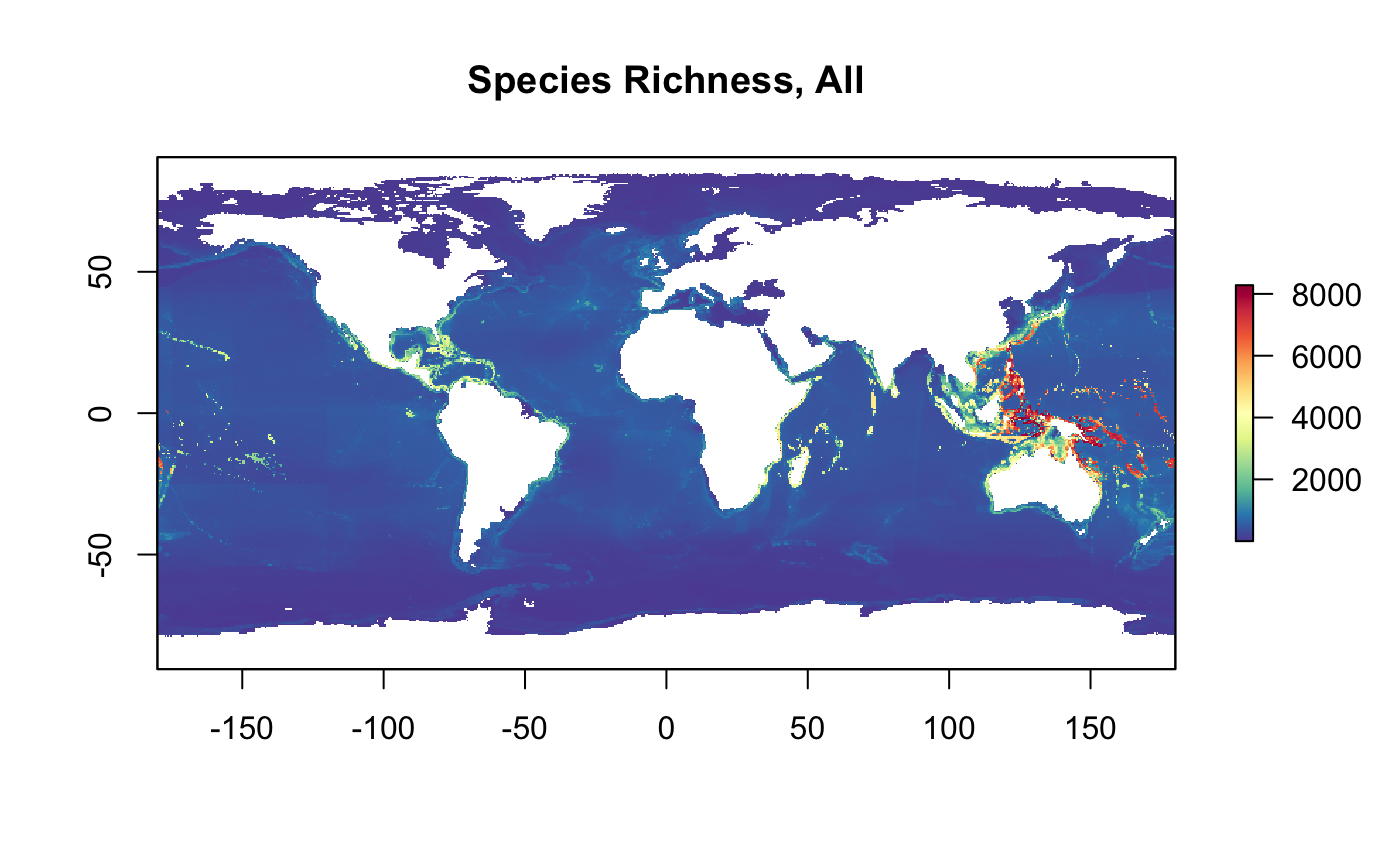

Calculate `nspp`, by taxonomic group

redo      <- F
spp       <- tbl(con, "spp")
cells     <- tbl(con, "cells")
spp_cells <- tbl(con, "spp_cells")

spp_groups <- tbl(con, "spp") %>% 
  arrange(group) %>% 
  distinct(group) %>% 
  pull(group)

for (i in seq_along(spp_groups)){
  group <- spp_groups[i]
  grp   <- group_to_grp(group)
  tif   <- (glue("{dir_out}/nspp_{grp}.tif"))
  
  if (file.exists(tif) & !redo) next()
  
  cat(glue("{str_pad(i, 2, pad='0')} of {length(spp_groups)}: {grp} - {Sys.time()}\n\n"))

  # get species diversity, with default col_cellid="cellid"
  if (is.na(group)){
    spp_grp <- filter(spp, is.na(group))
  } else{
    spp_grp <- filter(spp, group == !!group)
  }
  
  cells_nspp <- spp_grp %>% 
    select(SPECIESID) %>% 
    left_join(
      spp_cells %>% 
        select(
          SpeciesID, probability,
          CenterLat, CenterLong) %>% 
        filter(
          probability >= spp_prob_threshold), 
      by=c("SPECIESID"="SpeciesID")) %>% 
    left_join(
      cells, 
      by=c("CenterLat","CenterLong")) %>% 
    group_by(cellid) %>% 
    summarize(
      nspp = n()) %>% 
    collect()
  r_grp <- df_to_raster(cells_nspp, "nspp", tif)
  plot(r_grp, col = cols, main=glue("nspp {group}"))
}

# get all tifs, except first one "nspp_all.tif"
tifs <- list.files(dir_out, "^nspp_.*.tif$", full.names = T)[-1]
s_nspp <- stack(tifs)
names(s_nspp) <- str_replace(names(s_nspp), "nspp_", "")
plot(s_nspp, col = cols)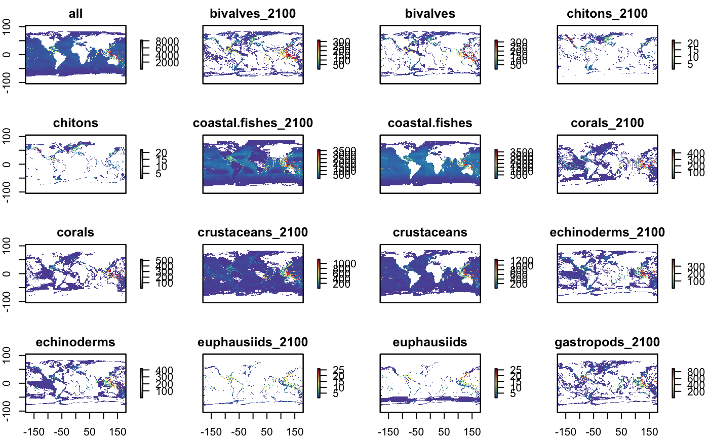

Calculate extinction risk

The Red List Index ((Butchart et al. 2007) et al. 2007) is summarized (Juslén et al. 2016) as:

The RLI [Red List Index] value was calculated by multiplying the number of taxa in each red-list category by the category weight (0 for LC, 1 for NT, 2 for VU, 3 for EN, 4 for CR, 5 for RE/EX). These products were summed and then divided by the number of taxa multiplied by the maximum weight 5 (“maximum possible denominator”). To obtain the RLI value, this sum is subtracted from 1. The index value varies between 0 and 1 (Butchart et al. 2007). The lower the value, the closer the set of taxa is heading towards extinction. If the value is 0 all the taxa are (regionally) extinct. If the value is 1 all the taxa are assessed as Least Concern.

We will use simply the numerator, the Red List Sum (RLS), of the Red List Index (RLI) to quantify the “endangeredness” of a cell without dilution from being in a species-rich place as the RLI does when averaging the extinction risk for all assessed species.

\[RLS = \sum_{i=1}^{n_{spp}} w_i\] \[RLI = 1 - \frac{RLS}{n_{spp} * max(w)}\]

Weights used for Red List Sum (RLS) indicator:

DD: NA - Data Deficient
LC: 0 - Least Concern
LR/lc: 0 - Lower Risk, least concern (1994 category)
NT: 1 - Near Threatened
LR/cd: 1 - Lower Risk, conservation dependent (1994 category)
LR/nt: 1 - Lower Risk, near threatened (1994 category)
VU: 2 - VUlnerable
EN: 3 - ENdangered
CR: 4 - CRitically endangered
EW: NA (*not 5) - Extinct in the Wild (n=0)
EX: NA (*not 5) - EXtinct (n=1)

Note that only 1 species is listed as extinct (EX) or extinct in the wild (EW). Since the species is no longer considered present, protection is assumed to not afford any conservation value.

Set `iucn_weight` to species

iucn_category_weights = c(
  DD=NA, 
  LC=0, `LR/lc`=0, 
  NT=1, `LR/cd`=1, `LR/nt`=1, 
  VU=2, 
  EN=3, 
  CR=4, 
  EW=NA,
  EX=NA)

spp_cols <- tbl(con, "spp") %>% head(1) %>% collect() %>% names()

if (!"iucn_weight" %in% spp_cols){
  
  spp <- tbl(con, "spp") %>% 
    collect() %>% 
    mutate(
      iucn_weight = recode(iucn_category, !!!iucn_category_weights))
  
  copy_to(
    con, spp, "spp", temporary=F, overwrite=T,
    unique_indexes=list("SPECIESID"),
    indexes = list("group", "genus_species", "iucn_weight"))
}

# save spp_csv
if (!file.exists(spp_csv)){
  tbl(con, "spp") %>% 
    collect() %>% 
    write_csv(spp_csv)
}

spp_iucn_weight <- tbl(con, "spp") %>% 
  pull(iucn_weight)
table(spp_iucn_weight, useNA="always")

## spp_iucn_weight
##     0     1     2     3     4  <NA> 
##  6187   314   379    87    42 17895

Calculate `rls`, all taxa

spp       <- tbl(con, "spp")
cells     <- tbl(con, "cells")
spp_cells <- tbl(con, "spp_cells")

tif <- (glue("{dir_out}/rls_all.tif"))

if (!file.exists(tif)){
  
  # calculate RedList sum of weights
  cells_rls <- spp %>% 
    filter(
      !is.na(iucn_weight), 
      iucn_weight != 0) %>% 
    left_join(
      spp_cells %>% 
        select(
          SpeciesID, probability,
          CenterLat, CenterLong) %>% 
        filter(
          probability >= spp_prob_threshold), 
      by=c("SPECIESID"="SpeciesID")) %>% 
    left_join(
      cells, by=c("CenterLat","CenterLong")) %>% 
    group_by(cellid) %>% 
    summarize(
      rls = sum(iucn_weight)) %>% 
    collect()
  r_rls_all <- df_to_raster(cells_rls, "rls", tif)
}

r_rls_all <- raster(tif)
plot(r_rls_all, col = cols, main="Red List Sum, All")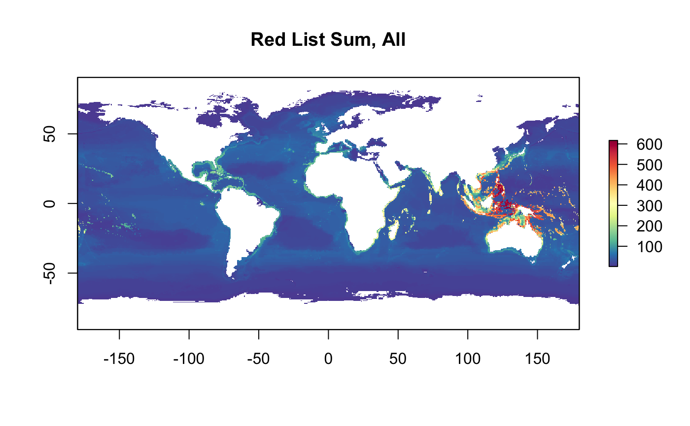

Calculate `rls`, by taxonomic group

redo      <- F
spp       <- tbl(con, "spp")
cells     <- tbl(con, "cells")
spp_cells <- tbl(con, "spp_cells")

spp_groups <- tbl(con, "spp") %>% 
  arrange(group) %>% 
  distinct(group) %>% 
  pull(group)

for (i in seq_along(spp_groups)){
  group <- spp_groups[i]
  grp   <- group_to_grp(group)
  tif   <- (glue("{dir_out}/rls_{grp}.tif"))
  
  if (file.exists(tif) & !redo) next()
  
  cat(glue("{str_pad(i, 2, pad='0')} of {length(spp_groups)}: {grp} - {Sys.time()}\n\n"))
  
  # filter by group
  if (is.na(group)){
    spp_grp <- filter(spp, is.na(group))
  } else{
    spp_grp <- filter(spp, group == !!group)
  }
  
  spp_grp_w <- spp_grp %>% 
    filter(
      !is.na(iucn_weight), 
      iucn_weight != 0) %>% 
    collect()
  
  if (nrow(spp_grp_w) == 0){
    #cat(glue("  all iucn_weight == NA\n", .trim=F))
  } else {
    # calculate RedList sum of weights
    cells_rls <- spp_grp %>% 
      filter(
        !is.na(iucn_weight), 
        iucn_weight != 0) %>% 
      left_join(
        spp_cells %>% 
          select(
            SpeciesID, probability,
            CenterLat, CenterLong) %>% 
          filter(
            probability >= spp_prob_threshold), 
        by=c("SPECIESID"="SpeciesID")) %>% 
      left_join(
        cells, by=c("CenterLat","CenterLong")) %>% 
      group_by(cellid) %>% 
      summarize(
        rls = sum(iucn_weight)) %>% 
      collect()
    
    r_grp <- df_to_raster(cells_rls, "rls", tif) 
    plot(r_grp, col = cols, main=glue("Red List Sum, {group}"))
  }
}

## 02 of 21: chitons - 2019-06-17 14:28:18
## 07 of 21: euphausiids - 2019-06-17 14:28:18
## 09 of 21: hydrozoans - 2019-06-17 14:28:18
## 10 of 21: mangroves - 2019-06-17 14:28:18
## 14 of 21: sea.spiders - 2019-06-17 14:28:18
## 15 of 21: seagrasses - 2019-06-17 14:28:18
## 17 of 21: sponges - 2019-06-17 14:28:18
## 19 of 21: tunicates - 2019-06-17 14:28:18
## 20 of 21: worms - 2019-06-17 14:28:18

# get all tifs, except first one "nspp_all.tif"
tifs <- list.files(dir_out, "^rls_.*.tif$", full.names = T)[-1]
s_rls <- stack(tifs)
names(s_rls) <- str_replace(names(s_rls), "rls_", "")
plot(s_rls, col = cols)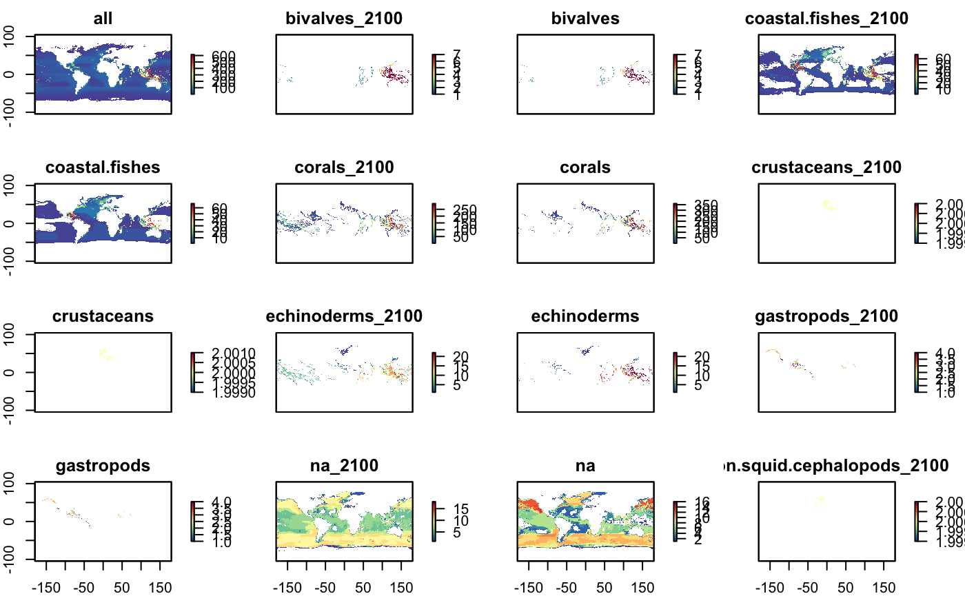

Climate Change Forecasts for 2100

The data from forecasting climate change effects on marine species distributions in 2050 using the AquaMaps model (Coro et al. 2016) were made publicly available through the server http://thredds.d4science.org and linked from AquaMaps species profiles.

TODO: resolve MISMATCH: - (Coro et al. 2016): 2050 - Aquamaps.org: 2100

To investigate accessing these data layers via iMarine, I logged into https://i-marine.d4science.org/group/biodiversitylab and see this entry:

Gianpaolo Coro Dear VRE Members,the AquaMaps Web site is now officially linked to D4Science! All automatically generated maps have links to download content in NetCDF format through D4Science and to interactively inspect the maps trough Web applications hosted by the e-Infrastructure. A total of 24,935 AquaMaps NetCDF files were produced for both today and 2100 through the DataMiner “Csv To NetCDF” conversion algorithms. Please, click on the link below to see an example for yellowback anthias and follow the “NetCDF” and the “view in Godiva” links on the page.

https://www.aquamaps.org/preMap2.php?cache=1&SpecID=Fis-10199

Following this link leads to:

http://thredds.d4science.org/thredds/fileServer/public/netcdf/AquaMaps_08_2016/Pseudanthias_evansi.nc

Computer Generated Native Distribution Map for {sp}, with modelled year 2100 native range map based on IPCC A2 emissions scenario
Cite this set of maps as: Computer generated distribution maps for {Genus} {species} ({common}), with modelled year 2100 native range map based on IPCC A2 emissions scenario. www.aquamaps.org, version of Aug. 2016. Web. Accessed 10 Jun. 2019.

library(raster)
library(glue)
library(here)

get_am2100nc <- function(sp, nc){
  # sp <- "Acanthopagrus_berda"
  # nc <- file.path(dir_nc, basename(url)) # unlink(nc)
  
  # get netcdf file
  url <- glue("http://thredds.d4science.org/thredds/fileServer/public/netcdf/AquaMaps_08_2016/{sp}.nc")
  
  if (file.exists(nc)) return (glue("{sp}: already exists"))
  tryCatch(
    download.file(url, nc, mode = "wb", quiet = T),
    error=function(e) e)
  return (glue("{sp}: {ifelse(file.exists(nc), 'downloaded', 'missing')}"))
    #spp_2100 <- spp_2100 %>% 
    #  mutate(
    #    downloaded = ifelse(sp_str == sp, file.exists(nc), downloaded))
    # head(spp_2100)
  #sp_downloaded <- filter(spp_2100, sp_str == sp) %>% pull(downloaded)
  #return(glue("{sp}: {sp_downloaded}"))
}

if (!file.exists(spp_2100_csv)){
  # get all species
  spp_2100 <- spp %>% 
    select(SPECIESID, Genus, Species) %>% 
    collect() %>% 
    mutate(
      sp_str     = glue("{Genus}_{Species}"),
      path_nc    = glue("{dir_nc}/{sp_str}.nc"),
      downloaded = NA) %>% 
    arrange(sp_str) # n= 24,894

  plan(multiprocess)
  
  # iterate in chunks of 1000
  n <- 1000
  for ( i in seq(1, nrow(spp_2100), by=n) ){ # i = 1
    
    i_beg <- i
    i_end <- i - 1 + n
    csv <- glue("{dirname(dir_nc)}/spp_2100_{str_pad(i_beg, 5, 'left', '0')}-{str_pad(i_end, 5, 'left', '0')}.csv")
    cat(glue("{basename(csv)} - {Sys.time()}\n\n"))
    
    # speed up fetching by running in parallel
    future_map2_chr(
      spp_2100$sp_str[i_beg:i_end], 
      spp_2100$path_nc[i_beg:i_end],
      get_am2100nc)
    
    # record species searched and not found
    spp_i <- slice(spp_2100, i_beg:i_end) %>%  
      mutate(
        downloaded = file.exists(path_nc)) # View(spp_i)
    write_csv(spp_i, csv)
  }
  
  # combine temporary csvs
  csvs <- list.files(dirname(dir_nc), "*\\.csv", full.names = T)
  spp_df <- map_df(csvs, read_csv) %>% dplyr::bind_rows() %>% 
    filter(!duplicated(sp_str))
  write_csv(spp_df, spp_2100_csv)
  unlink(csvs)
}

# quickfix
# spp_df2 <- spp_df %>% 
#   left_join(
#     spp_2100 %>% 
#       select(sp_str, SPECIESID),
#     by="sp_str") %>% 
#   select(SPECIESID, Genus, Species, sp_str, path_nc, downloaded)
# write_csv(spp_df2, spp_2100_csv)


if (!"spp_cells_2100" %in% dbListTables(con)){
  
  dbExecute(con, 'CREATE TABLE spp_cells_2100 (
  speciesid text,
  cellid int4,
  probability float8);
  CREATE UNIQUE INDEX idx_spp_cells_2100_unique ON spp_cells_2100 (speciesid, cellid);')
  
  r_na   <- raster_na()
  spp_df <- read_csv(spp_2100_csv) %>% 
    filter(downloaded) # 24894 - 24831 = 63 unavailable
  # of 24,894 spp: 63 unavailable, 20 mismatch and 5 unreadable

  #for (i in 1:nrow(spp_df)){ # i = 1087
  for (i in 18009:nrow(spp_df)){ # i = 18009
    if (i %% 1000 == 0) cat(glue("{sprintf('%06d',i)} - {Sys.time()}\n\n"))
    
    nc    <- spp_df$path_nc[i]
    sp_id <- spp_df$SPECIESID[i]
    
    #r <- raster(nc, varname="probability")
    r <- tryCatch(raster(nc, varname="probability"),
      error = function(e) cat(glue(
        "  can't read {sprintf('%06d',i)} {sp_id} {basename(nc)} - {Sys.time()}\n\n")))
    if (is.null(r)) next
    
    tryCatch(
      compareRaster(
        r, r_na, 
        extent=F, rowcol=F, 
        crs=T, res=T, orig=T, rotation=T),
      error = function(e) cat(glue(
        "  mismatch {sprintf('%06d',i)} {sp_id} {basename(nc)} - {Sys.time()}\n\n")))
    # i = 1087  # 2019-06-10 00:03:23
    # Error in compareRaster(): different resolution
    #   extent      : -81, -78, -37.5, -15  (xmin, xmax, ymin, ymax)
    #   data source : /Users/bbest/docker_pg_data/aquamaps2100_nc/Amphichaetodon_melbae.nc 
    # mismatch 001087 Fis-33857 Amphichaetodon_melbae.nc - 2019-06-10 00:15:56
    # mismatch 001433 URM-2-1014 Anoplodactylus_laminifer.nc - 2019-06-10 00:17:01
    # mismatch 003352 Fis-144824 Bovichtus_veneris.nc - 2019-06-10 00:23:45
    # mismatch 004814 NZ-24280 Charitometra_incisa.nc - 2019-06-10 00:28:13
    # mismatch 005270 Fis-60663 Chromis_pamae.nc - 2019-06-10 00:29:39
    # mismatch 007885 Fis-147877 Ebinania_macquariensis.nc - 2019-06-10 00:37:37
    # mismatch 009752 Fis-27991 Genicanthus_semicinctus.nc - 2019-06-10 00:42:44
    # mismatch 009852 Fis-134861 Girella_albostriata.nc - 2019-06-10 00:43:03
    # mismatch 011115 URM-2-3593 Heterostigma_singulare.nc - 2019-06-10 00:46:36
    # mismatch 011989 ITS-552955 Jasus_paulensis.nc - 2019-06-10 00:49:06
    # mismatch 012027 W-Iso-256075 Joeropsis_sanctipauli.nc - 2019-06-10 00:49:11
    # mismatch 014326 SLB-142070 Microdictyon_okamurae.nc - 2019-06-10 00:55:57
    # mismatch 015881 Fis-168180 Novaculops_koteamea.nc - 2019-06-10 06:00:43
    # mismatch 016386 Fis-130905 Ophichthus_kunaloa.nc - 2019-06-10 06:02:24
    # mismatch 016430 Fis-133519 Ophidion_metoecus.nc - 2019-06-10 06:02:30
    # mismatch 017495 Fis-123220 Parapercis_dockinsi.nc - 2019-06-10 06:05:43
    # mismatch 020940 Fis-153727 Scartella_poiti.nc - 2019-06-10 07:21:30
    # mismatch 020942 Fis-61194 Scartichthys_variolatus.nc - 2019-06-10 07:21:30
    # mismatch 022003 Fis-164212 Sparisoma_rocha.nc - 2019-06-10 07:24:20
    # mismatch 023107 URM-2-336 Tanystylum_beuroisi.nc - 2019-06-10 07:27:33
    # mismatch rasters: n=20
    
    # i = 17793 Patagonotothen_sima.nc
    # Error in .local(x, ...) : min and max x are the same
    # 128-111-61-209:aquamaps2100_nc bbest$ gdalinfo Patagonotothen_sima.nc
    # Warning 1: No UNIDATA NC_GLOBAL:Conventions attribute
    # Driver: netCDF/Network Common Data Format
    # Files: Patagonotothen_sima.nc
    # Size is 512, 512
    # Coordinate System is `'
    # Subdatasets:
    #   SUBDATASET_1_NAME=NETCDF:"Patagonotothen_sima.nc":probability
    #   SUBDATASET_1_DESC=[107x66] probability (64-bit floating-point)
    #   SUBDATASET_2_NAME=NETCDF:"Patagonotothen_sima.nc":faoareayn
    #   SUBDATASET_2_DESC=[107x66] faoareayn (32-bit integer)
    #   SUBDATASET_3_NAME=NETCDF:"Patagonotothen_sima.nc":boundboxyn
    #   SUBDATASET_3_DESC=[107x66] boundboxyn (32-bit integer)
    # Corner Coordinates:
    # Upper Left  (    0.0,    0.0)
    # Lower Left  (    0.0,  512.0)
    # Upper Right (  512.0,    0.0)
    # Lower Right (  512.0,  512.0)
    # Center      (  256.0,  256.0)
    # can't read 17793 ? Patagonotothen_sima.nc
    # can't read 018009 ITS-612391 Periclimenes_brevicarpalis.nc - 2019-06-10 07:12:45
    # can't read 018176 W-Por-246569 Phakellia_columnata.nc - 2019-06-10 07:13:18
    # can't read 018009 ITS-612391 Periclimenes_brevicarpalis.nc - 2019-06-10 07:12:45
    # can't read 018176 W-Por-246569 Phakellia_columnata.nc - 2019-06-10 07:13:18
    # can't read rasters: n=5    
    
    #r <- extend(r, r_na)
    r <- raster::projectRaster(r, r_na)
    d <- tibble(
      speciesid = sp_id,
      probability = raster::values(r)) %>% 
      tibble::rowid_to_column(var = "cellid") %>% 
      filter(!is.na(probability))
    
    #dbExecute(con, glue("DELETE FROM spp_cells_2100;"))
    dbExecute(con, glue("DELETE FROM spp_cells_2100 WHERE SpeciesID='{sp_id}';"))
    dbWriteTable(con, "spp_cells_2100", d, append=T, row.names=F)
  }
  # i = 1
}

Calculate species richness

Calculate `nspp`, all taxa

spp_prob_threshold <- 0.5

spp       <- tbl(con, "spp")
cells     <- tbl(con, "cells")
spp_cells <- tbl(con, "spp_cells_2100")

tif <- (glue("{dir_out}/nspp_all_2100.tif"))

if (!file.exists(tif)){
  
  # get species richness, with default col_cellid="cellid"
  cells_nspp <- spp_cells %>% 
    filter(
      probability >= spp_prob_threshold) %>% 
    group_by(cellid) %>% 
    summarize(
      nspp = n()) %>% 
    collect()
  r_nspp_all_2100 <- df_to_raster(cells_nspp, "nspp", tif)
}

r_nspp_all_2100 <- raster(tif)

plot(r_nspp_all_2100, col = cols, main="Species Richness, All 2100")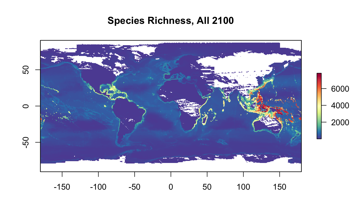

Calculate `nspp`, by taxonomic group

redo      <- F
#options(warn=2) # error on warning
spp       <- tbl(con, "spp")
cells     <- tbl(con, "cells")
spp_cells <- tbl(con, "spp_cells_2100")

spp_groups <- tbl(con, "spp") %>% 
  arrange(group) %>% 
  distinct(group) %>% 
  pull(group)

for (i in seq_along(spp_groups)){ # i = 1
  group <- spp_groups[i]
  grp   <- group_to_grp(group)
  tif   <- (glue("{dir_out}/nspp_{grp}_2100.tif"))
  
  if (file.exists(tif) & !redo) next()
  
  cat(glue("{str_pad(i, 2, pad='0')} of {length(spp_groups)}: {grp} - {Sys.time()}\n\n"))

  # get species diversity, with default col_cellid="cellid"
  if (is.na(group)){
    spp_grp <- filter(spp, is.na(group))
  } else{
    spp_grp <- filter(spp, group == !!group)
  }
  
  cells_nspp_2100 <- spp_grp %>% 
    select(SPECIESID) %>% 
    left_join(
      spp_cells %>% 
        select(
          speciesid, cellid, probability) %>% 
        filter(
          probability >= spp_prob_threshold), 
      by=c("SPECIESID"="speciesid")) %>% 
    group_by(cellid) %>% 
    summarize(
      nspp = n()) %>% 
    collect()
  r_grp_2100 <- df_to_raster(cells_nspp_2100, "nspp", tif)
  plot(r_grp_2100, col = cols, main=glue("nspp {group} 2100"))
}

# get all tifs, except first one "nspp_all_2100.tif"
tifs   <- list.files(dir_out, "^nspp_.*_2100\\.tif$", full.names = T)[-1]
s_nspp_2100 <- stack(tifs)
names(s_nspp_2100) <- names(s_nspp_2100) %>% 
  str_replace("nspp_", "") %>% 
  str_replace("_2100", "")
plot(s_nspp_2100, col = cols)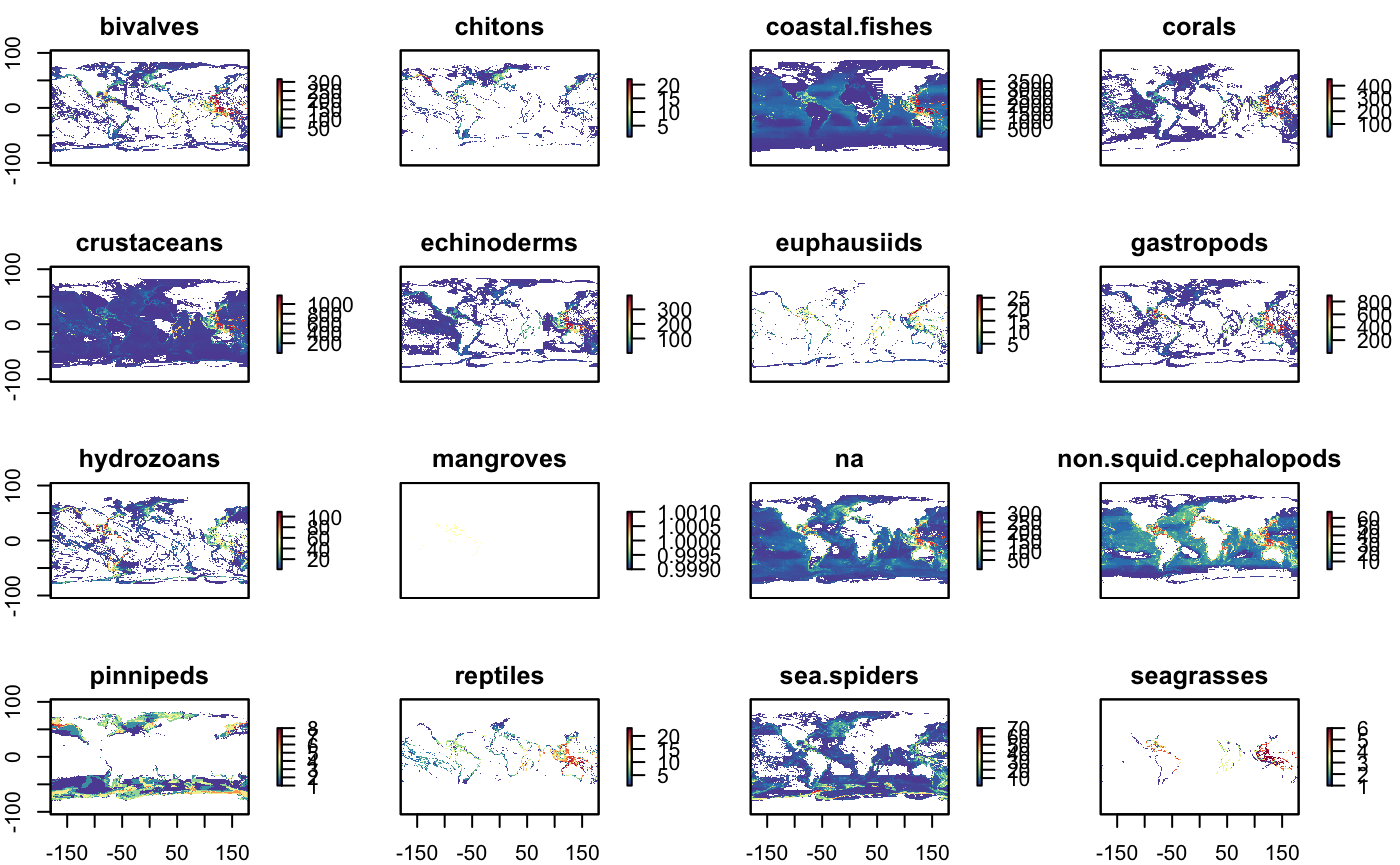

Calculate extinction risk

Calculate `rls`, all taxa

spp       <- tbl(con, "spp")
cells     <- tbl(con, "cells")
spp_cells <- tbl(con, "spp_cells_2100")

tif <- (glue("{dir_out}/rls_all_2100.tif"))

if (!file.exists(tif)){
  
  # calculate RedList sum of weights
  cells_rls_2100 <- spp %>% 
    filter(
      !is.na(iucn_weight), 
      iucn_weight != 0) %>% 
    left_join(
      spp_cells %>% 
        select(
          speciesid, cellid, probability) %>% 
        filter(
          probability >= spp_prob_threshold), 
      by=c("SPECIESID"="speciesid")) %>% 
    group_by(cellid) %>% 
    summarize(
      rls = sum(iucn_weight, na.rm=T)) %>% 
    collect()
  r_rls_all_2100 <- df_to_raster(cells_rls_2100, "rls", tif)
}

r_rls_all_2100 <- raster(tif)
plot(r_rls_all_2100, col = cols, main="Red List Sum, All 2100")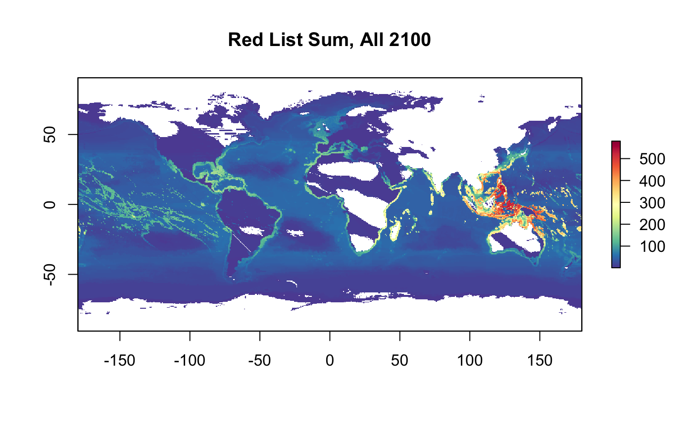

Calculate `rls`, by taxonomic group

redo      <- F
spp       <- tbl(con, "spp")
cells     <- tbl(con, "cells")
spp_cells <- tbl(con, "spp_cells_2100")

spp_groups <- tbl(con, "spp") %>% 
  arrange(group) %>% 
  distinct(group) %>% 
  pull(group)

for (i in seq_along(spp_groups)){ # i = 1
  group <- spp_groups[i]
  grp   <- group_to_grp(group)
  tif   <- (glue("{dir_out}/rls_{grp}_2100.tif"))
  
  if (file.exists(tif) & !redo) next()
  
  cat(glue("{str_pad(i, 2, pad='0')} of {length(spp_groups)}: {grp} - {Sys.time()}\n\n"))
  
  # filter by group
  if (is.na(group)){
    spp_grp <- filter(spp, is.na(group))
  } else{
    spp_grp <- filter(spp, group == !!group)
  }
  
  spp_grp_w <- spp_grp %>% 
    filter(
      !is.na(iucn_weight), 
      iucn_weight != 0) %>% 
    collect()
  
  if (nrow(spp_grp_w) == 0){
    cat(glue("  all iucn_weight == NA\n", .trim=F))
  } else {
    # calculate RedList sum of weights
    cells_rls_2100 <- spp_grp %>% 
      filter(
        !is.na(iucn_weight), 
        iucn_weight != 0) %>% 
      left_join(
        spp_cells %>% 
          select(
            speciesid, cellid, probability) %>% 
          filter(
            probability >= spp_prob_threshold), 
        by=c("SPECIESID"="speciesid")) %>% 
      group_by(cellid) %>% 
      summarize(
        rls = sum(iucn_weight, na.rm = T)) %>% 
      collect()
    
    r_grp_2100 <- df_to_raster(cells_rls_2100, "rls", tif) 
    plot(r_grp_2100, col = cols, main=glue("Red List Sum, {group} 2100"))
  }
}

## 02 of 21: chitons - 2019-06-17 14:28:26
##   all iucn_weight == NA
## 07 of 21: euphausiids - 2019-06-17 14:28:27
##   all iucn_weight == NA
## 09 of 21: hydrozoans - 2019-06-17 14:28:27
##   all iucn_weight == NA
## 10 of 21: mangroves - 2019-06-17 14:28:27
##   all iucn_weight == NA
## 14 of 21: sea.spiders - 2019-06-17 14:28:27
##   all iucn_weight == NA
## 15 of 21: seagrasses - 2019-06-17 14:28:27
##   all iucn_weight == NA
## 17 of 21: sponges - 2019-06-17 14:28:27
##   all iucn_weight == NA
## 19 of 21: tunicates - 2019-06-17 14:28:27
##   all iucn_weight == NA
## 20 of 21: worms - 2019-06-17 14:28:27
##   all iucn_weight == NA

# get all tifs, except first one "rls_all_2100.tif"
tifs   <- list.files(dir_out, "^rls_.*_2100\\.tif$", full.names = T)[-1]
s_rls_2100 <- stack(tifs)
names(s_rls_2100) <- names(s_rls_2100) %>% 
  str_replace("rls_", "") %>% 
  str_replace("_2100", "")
plot(s_rls_2100, col = cols)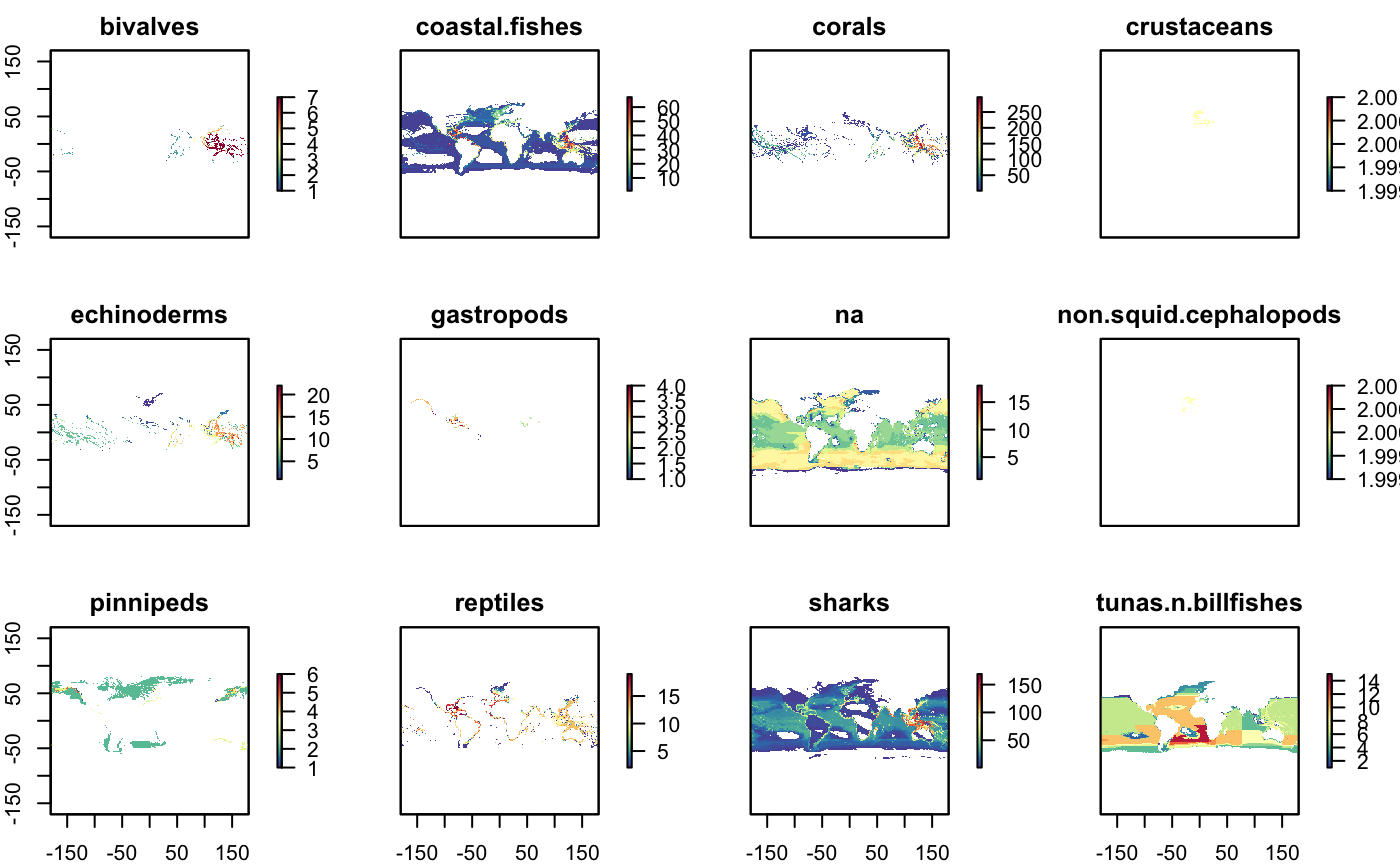

TODO: Archive DB

## TODO: Archive db

# [arkdb](https://ropensci.github.io/arkdb/): archive and unarchive databases using flat files

References

Butchart, Stuart H. M., H. Resit Akçakaya, Janice Chanson, Jonathan E. M. Baillie, Ben Collen, Suhel Quader, Will R. Turner, Rajan Amin, Simon N. Stuart, and Craig Hilton-Taylor. 2007. “Improvements to the Red List Index.” PLOS ONE 2 (1): e140. doi:10.1371/journal.pone.0000140.

Coro, Gianpaolo, Chiara Magliozzi, Anton Ellenbroek, Kristin Kaschner, and Pasquale Pagano. 2016. “Automatic Classification of Climate Change Effects on Marine Species Distributions in 2050 Using the AquaMaps Model.” Environ Ecol Stat 23 (1): 155–80. doi:10.1007/s10651-015-0333-8.

Juslén, Aino, Juha Pykälä, Saija Kuusela, Lauri Kaila, Jaakko Kullberg, Jaakko Mattila, Jyrki Muona, Sanna Saari, and Pedro Cardoso. 2016. “Application of the Red List Index as an Indicator of Habitat Change.” Biodivers Conserv 25 (3): 569–85. doi:10.1007/s10531-016-1075-0.

Kaschner, K., K. Kesner-Reyes, C. Garilao, J. Rius-Barile, T. Rees, and R. Froese. 2016. “AquaMaps: Predicted Range Maps for Aquatic Species.” World Wide Web Electronic Publication.

Klein, Carissa J., Christopher J. Brown, Benjamin S. Halpern, Daniel B. Segan, Jennifer McGowan, Maria Beger, and James E. M. Watson. 2015. “Shortfalls in the Global Protected Area Network at Representing Marine Biodiversity.” Scientific Reports 5 (December): 17539. doi:10.1038/srep17539.

O’Hara, Casey C., Jamie C. Afflerbach, Courtney Scarborough, Kristin Kaschner, and Benjamin S. Halpern. 2017. “Aligning Marine Species Range Data to Better Serve Science and Conservation.” PLOS ONE 12 (5): e0175739. doi:10.1371/journal.pone.0175739.

Tittensor, Derek P., Camilo Mora, Walter Jetz, Heike K. Lotze, Daniel Ricard, Edward Vanden Berghe, and Boris Worm. 2010. “Global Patterns and Predictors of Marine Biodiversity Across Taxa.” Nature 466 (7310): 1098–1101. doi:10.1038/nature09329.

Ben Best

2019-06-17

Setup database

create volume pg_data

create container postgis, database am user admin

Connect to database

Load AquaMaps csvs into database

Assign taxonomic groups

Get extinction risk from IUCN

Calculate species richness

Calculate nspp, all taxa

Calculate nspp, by taxonomic group

Calculate extinction risk

Set iucn_weight to species

Calculate rls, all taxa

Calculate rls, by taxonomic group

Climate Change Forecasts for 2100

Calculate species richness

Calculate nspp, all taxa

Calculate nspp, by taxonomic group

Calculate extinction risk

Calculate rls, all taxa

Calculate rls, by taxonomic group

TODO: Archive DB

References

Contents

create volume `pg_data`

create container `postgis`, database `am` user `admin`

Calculate `nspp`, all taxa

Calculate `nspp`, by taxonomic group

Set `iucn_weight` to species

Calculate `rls`, all taxa

Calculate `rls`, by taxonomic group

Calculate `nspp`, all taxa

Calculate `nspp`, by taxonomic group

Calculate `rls`, all taxa

Calculate `rls`, by taxonomic group