Observations
Species with most OBIS observations. Later try temporally subsetting to look for migratory patterns. And run for all.
Environment
Environmental data from sdmpredictors. Need to know whether demersal or pelagic. For now extract static climatic environmental predictors for model fitting and prediction. Later extract dynamic predictors synchronous in time for model fitting and predict with hind-/now-/fore-cast or climatic seasonal snapshot.
Warning: package 'arrow' was built under R version 4.3.1
Warning: package 'leafem' was built under R version 4.3.1
options(readr.show_col_types = F)# variables -----dir_data <-"/Users/bbest/My Drive/projects/mbon-sdm/data"obis_prq <-glue("{dir_data}/raw/obis.org/obis_20230726.parquet")# functions -----get_sp_occ_obis_prq <-function( aphia_id,obis_prq ="/Users/bbest/My Drive/projects/mbon-sdm/data/raw/obis.org/obis_20230726.parquet",cols_keep =c("id","phylum","class","taxonRank","scientificName","AphiaID","date_mid","decimalLongitude","decimalLatitude","depth","individualCount","flags")) {# get species occurrences from OBIS parquet file# TODO: add caching per species request/args# return only observations with valid coordinates and year o <-open_dataset(obis_prq) |>filter(!is.na(date_mid),!is.na(decimalLongitude),!is.na(decimalLatitude), AphiaID ==!!aphia_id) |>select(all_of(cols_keep)) |>collect() |>mutate(date_mid =as.POSIXct( date_mid/1000, origin ="1970-01-01",tz ="GMT") |>as.Date()) |>st_as_sf(coords =c("decimalLongitude", "decimalLatitude"), crs =4326)}
Species candidates
# species with most observationssp_gull <-read_csv("data/obis_top-species.csv") |>arrange(desc(n_obs)) |>slice(1)# non-bird species with most observationssp_herring <-read_csv("data/obis_top-species.csv") |>filter(class !="Aves") |>arrange(desc(n_obs)) |>slice(1)# species with ~100 observations (and most in Class)sp_jelly <-read_csv("data/obis_top-species.csv") |>filter(n_obs >240) |>arrange(n_obs) |>slice(1)
# right whale: surface, migratory, endangeredsp_rwhale <-tibble(AphiaID =159023)# prep single species observations ---sp <- sp_rwhaleaphia_id <- sp$AphiaID# get observationsobs <-get_sp_occ_obis_prq(aphia_id)obs
Simple feature collection with 7359 features and 10 fields
Geometry type: POINT
Dimension: XY
Bounding box: xmin: -93.3655 ymin: -33.88334 xmax: 153.56 ymax: 71.38
Geodetic CRS: WGS 84
# A tibble: 7,359 × 11
id phylum class taxonRank scientificName AphiaID date_mid depth
* <chr> <chr> <chr> <chr> <chr> <int> <date> <dbl>
1 0096eb8c-eeaf… Chord… Mamm… Species Eubalaena gla… 159023 2017-06-15 NA
2 00be3393-fc00… Chord… Mamm… Species Eubalaena gla… 159023 2003-09-02 NA
3 00edac0b-4e7b… Chord… Mamm… Species Eubalaena gla… 159023 2002-08-27 NA
4 00f04c3a-702e… Chord… Mamm… Species Eubalaena gla… 159023 2020-09-13 NA
5 00f344c2-7c0e… Chord… Mamm… Species Eubalaena gla… 159023 2002-08-23 NA
6 011cda0b-d2c8… Chord… Mamm… Species Eubalaena gla… 159023 2019-08-24 NA
7 01ad0d52-7c61… Chord… Mamm… Species Eubalaena gla… 159023 2017-03-06 NA
8 02198ff2-acde… Chord… Mamm… Species Eubalaena gla… 159023 1998-09-12 NA
9 021bb218-68d1… Chord… Mamm… Species Eubalaena gla… 159023 2003-08-31 NA
10 0220a6b3-6738… Chord… Mamm… Species Eubalaena gla… 159023 2018-05-31 NA
# ℹ 7,349 more rows
# ℹ 3 more variables: individualCount <chr>, flags <chr>, geometry <POINT [°]>
The 'cran_repo' argument in shelf() was not set, so it will use
cran_repo = 'https://cran.r-project.org' by default.
To avoid this message, set the 'cran_repo' argument to a CRAN
mirror URL (see https://cran.r-project.org/mirrors.html) or set
'quiet = TRUE'.
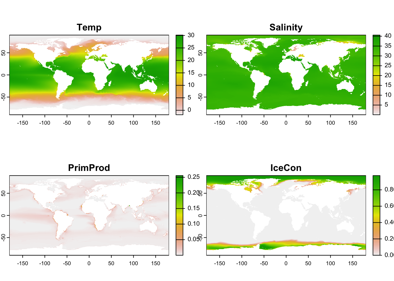
# see ../aquamaps-downscaled/index.qmd for creationenv_tif <-here("../aquamaps-downscaled/data/bio-oracle.tif")stopifnot(file.exists(env_tif))env <-rast(env_tif)names(env) <-c("Temp","Salinity","PrimProd","IceCon")plot(env)
Warning: package 'predicts' was built under R version 4.3.1
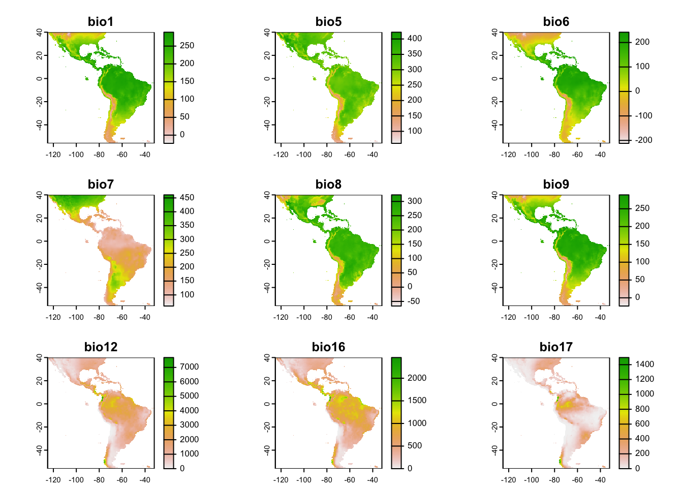
#?predicts::MaxEnt# MaxEnt()# This is MaxEnt_model version 3.4.3# get predictor variablesf <-system.file("ex/bio.tif", package="predicts")preds <-rast(f)plot(preds)
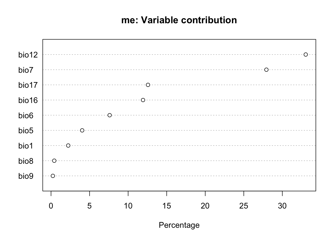
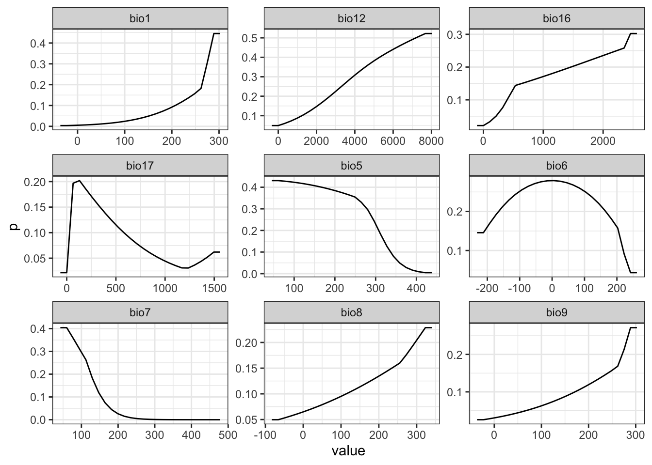
# file with presence pointsoccurence <-system.file("/ex/bradypus.csv", package="predicts")occ <-read.csv(occurence)[,-1]# witholding a 20% sample for testing fold <-folds(occ, k=5)occtest <- occ[fold ==1, ]occtrain <- occ[fold !=1, ]# fit modelme <-MaxEnt(preds, occtrain)# see the MaxEnt results in a browser:# medir_copy(attr(me, "path"), here("me_bradypus"))
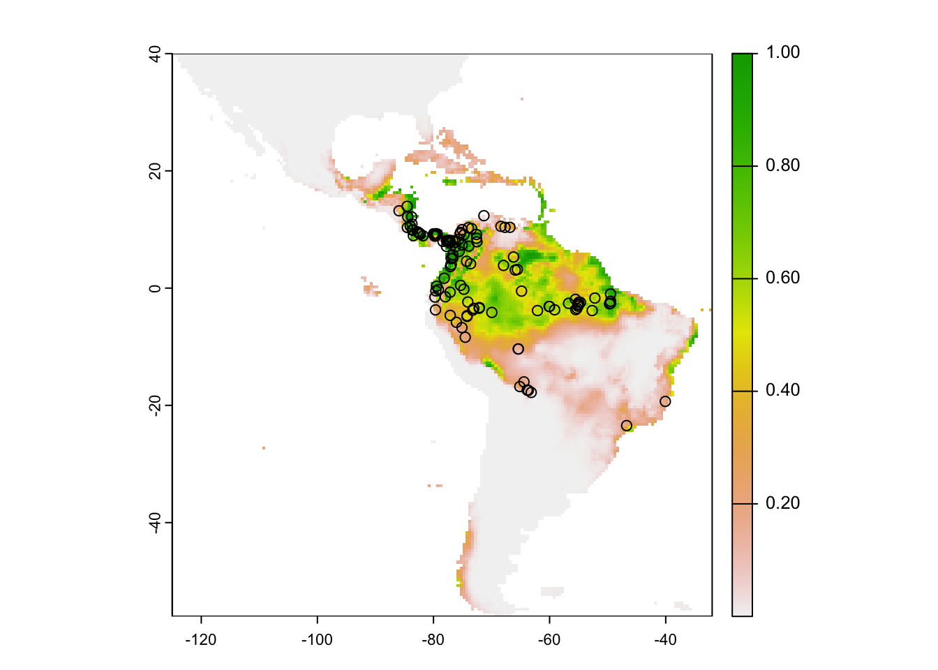
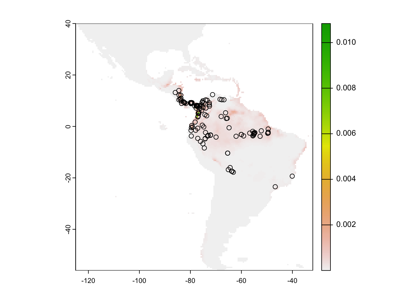
# with some options:r <-predict(me, preds, args=c("outputformat=raw"))plot(r)points(occ)
rwhale
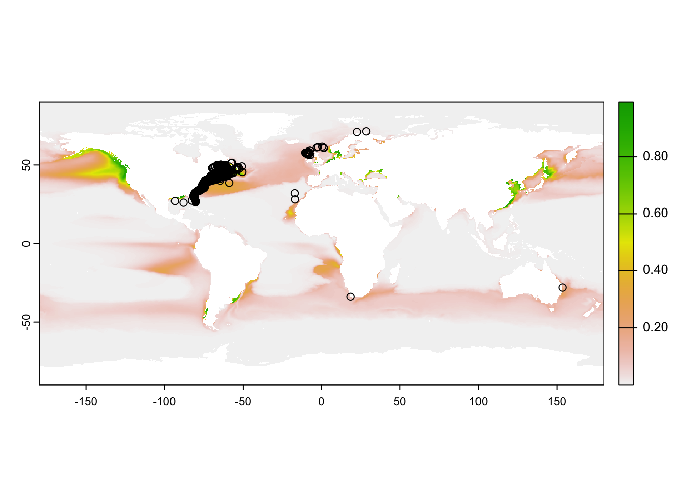
# get predictor variablespreds <- envplot(preds)
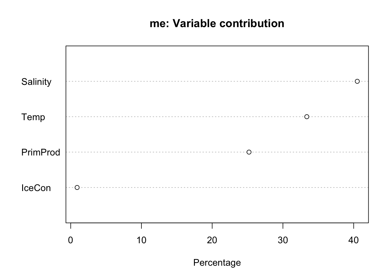
# witholding a 20% sample for testing occ <- obs |>mutate(lon =st_coordinates(geometry)[,1],lat =st_coordinates(geometry)[,2]) |>st_drop_geometry() |>select(lon, lat)fold <-folds(occ, k=5)occtest <- occ[fold ==1, ]occtrain <- occ[fold !=1, ]# fit modelsystem.time({ me <-MaxEnt(preds, occtrain)})
Warning in .local(x, p, ...): 2 (0.12%) of the presence points have NA
predictor values
user system elapsed
78.814 0.707 79.593
# Warning message:# In .local(x, p, ...) :# 3 (0.19%) of the presence points have NA predictor values# see the MaxEnt results in a browser:# see the MaxEnt results in a browser:# medir_copy(attr(me, "path"), here("me_rwhale"))